• Analytics Blog
LAST UPDATED
April 21, 2021
Data Golf predictive model: methodology
- November 22, 2018
[Contents:
Introduction,
Adjusting scores,
Predicting scores using total strokes-gained,
Incorporating detailed strokes-gained categories,
Course history/fit,
Model selection,
Adapting model for live predictions]
Introduction
In this document we describe the current methodology behind our predictive model and
discuss some interesting ideas and problems with prediction in golf more generally.
We have previously written about our first attempt at modelling golf
here,
which I would recommend reading but is not necessary to follow the contents of this article. This document
is a little more technical than the previous one, so if you are struggling to follow along here it is probably
worth reading the first methodology blog.
The goal of this prediction exercise is to estimate probabilities of certain finish positions in golf tournaments (e.g. winning, finishing in the top 10). We are going to obtain these estimates by specifying a probability distribution for each golfer's scores. With those distributions in hand, the probability of any tournament result can be estimated through simulation. Let's dig in to the details.
The goal of this prediction exercise is to estimate probabilities of certain finish positions in golf tournaments (e.g. winning, finishing in the top 10). We are going to obtain these estimates by specifying a probability distribution for each golfer's scores. With those distributions in hand, the probability of any tournament result can be estimated through simulation. Let's dig in to the details.
To build intuition, we can think of modelling each golfer's performance as normally
distributed with some unknown mean and variance. (In practice, we allow scores to follow a flexible
distribution, as they are not quite normal [1].)
These means can be thought of as the current "ability" of each golfer. Performance in golf is
only meaningful in relation to other golfers: a 72 on one golf course could indicate
a very different performance than a 72 on a different course. Therefore, throughout this analysis
we focus on an adjusted strokes-gained
measure (i.e. how many strokes better you were than some benchmark) that allows for direct comparisons of performance
on any course. To return to our simple probability model of a golfer's performance, we can
now more specifically say that we are modelling each golfer's adjusted strokes-gained
in a given round.
An obvious, but critical, point is that our measure of performance is in units
of strokes per round. Strokes relative-to-the field are the currency of the game of golf: this
decides who wins golf tournaments. If we can accurately
specify each golfer's probability distribution of strokes-gained relative to some
benchmark, then we can accurately estimate probabilities of certain
events occuring in golf tournaments.
Adjusting Scores
The overall approach we take can be broken down as follows: first, we adjust raw scores from all professional golf tournaments
to obtain a measure of performance that is not confounded by the difficulty of the course it was played on. Second,
we use various statistical methods to estimate the player-specific means and variances (mentioned above) using all available data before
a round is played. Third and finally, we use these estimates to simulate golf tournaments and obtain the probabilities of interest.
Let's talk first about how to convert a set of raw scores into the more interpretable adjusted strokes-gained measure.
The approach we take roughly follows
Connolly and Rendleman (2008). We estimate the following regression:
$$ \normalsize (1) \>\>\>\>\>\>\>\> S_{ij} = \mu_{i}(t) + \delta_{j} + \epsilon_{ij} $$
where i indexes the golfer and j indexes a tournament-round (or a round played
on a specific course for multi-course tournaments), \( \normalsize S_{ij} \) is the raw score in a given tournament-round,
\( \normalsize \mu_{i}(t) \) is some player-specific function of "golf time" (i.e. the sequence of rounds for a golfer), and
\( \normalsize \delta_{j} \) is the coefficient from a dummy variable for tournament-round j. This regression
produces estimates of each golfer's ability at each point in time (\( \normalsize \mu_{i}(t) \)) and of
the difficulty of each course in each tournament-round (\( \normalsize \delta_{j} \)). \( \normalsize \mu_{i}(t) \) could be any function:
one simple functional form could just be a constant, which would mean we force each player's ability
to be constant throughout our sample time period (a strong assumption). In practice, we fit second or third
order polynomials, depending how many data points the player has in our sample, which allows each golfer's ability
to vary flexibly over time.
All that we actually care about from this regression are the estimates
of course difficulty, as we define our adjusted strokes-gained measure as \( \normalsize S_{ij} - \delta_{j} \).
The interpretation of a single \( \normalsize \delta_{j} \) is the expected score for some reference
player at the course tournament-round j was played on. (More intuitively, \( \normalsize \delta_{j} \) can be
thought of as the field average score in round j after accounting for the skill of each golfer in
that field.) Therefore, our adjusted strokes-gained
measure is interpreted as the performance relative to that reference point. The choice of a
reference player is arbitrary and not of great importance, so we typically make everything
relative to the average PGA Tour player in a given year. A final point about this specification:
there are no course-player effects (i.e. players are not allowed to "match" better with certain courses
than others). With respect to obtaining consistent estimates of the \( \normalsize \delta_{j} \) (which is our only goal here), this is likely not too
important [2].
With our adjusted strokes-gained measure in hand, the next step is to estimate the golfer-specific parameters: the mean and the variance
of their scoring distributions (at each point in time).
It would seem that the function \( \normalsize \mu_{i}(t) \) would be a good candidate for an estimate
of the mean of player i's scoring distribution
[3]. It may be useful for some settings, but when your goal is
predicting out-of-sample, I don't think it is. Rather, we are going to estimate our player-specific means
using regression and backtesting.
It's worth noting that this method is not quite internally consistent. We require estimates of player ability
at each point in time to estimate the course difficulty parameters (\( \normalsize \delta_{j} \)), but we
do not actually use the player ability estimates from (1) to make predictions
[4].
You can think of the purpose of estimating (1) as only to recover the course difficulty parameters (\( \normalsize \delta_{j} \)),
from which we can calculate an adjusted strokes-gained measure for each round played in our sample.
The remainder of this document is concerned with how best
to predict these adjusted strokes-gained values with the available data at the time each round is played.
Predicting scores using historical total strokes-gained
In this section we give the overview of our predictive model and in the following two sections we
discuss the (potential) addition of a couple other features to the model.
The estimating sample includes data from 2004-onwards on the PGA, European, and Korn Ferry tours,
data from 2010-onwards on the remaining OWGR-sanctioned tours,
and amateur data from GolfStat and
WAGR since 2010.
We use a regression framework to predict a golfer's adjusted score in a
tournament-round using only information available up to that date. This seems to be a good fit
for our goals with this model (i.e. predicting out-of-sample), while you could maybe argue
the model in (1) would be better at describing data in-sample.
In this first iteration of the model, the main input to predict strokes-gained is a golfer's
historical strokes-gained (seems logical enough, right?). We expect that recent strokes-gained performances are more
relevant than performances further into the past, but we will let the data decide
whether and to what degree that is the case. For now, suppose we have a weighting scheme:
that is, each round a golfer has played moving back in time has been assigned a weight.
From this we construct a weighted average
and use that to predict a golfer's adjusted strokes-gained in their
next tournament-round. Also used to form these predictions are the number of rounds that
the weighted average is calcuated from, and the number of days since a golfer's last tournament-round.
More specifically, predictions are the fitted values from a regression of adjusted strokes-gained
in a given round on the set of predictors (weighted average SG up to that point in time,
rounds played up to that point in time, days since last tournament-round) and various interactions of these predictors.
The figure below summarizes the predictions the model makes: we plot fitted values as a function of how many rounds a golfer has played
for a few different values of the weighted strokes-gained average:
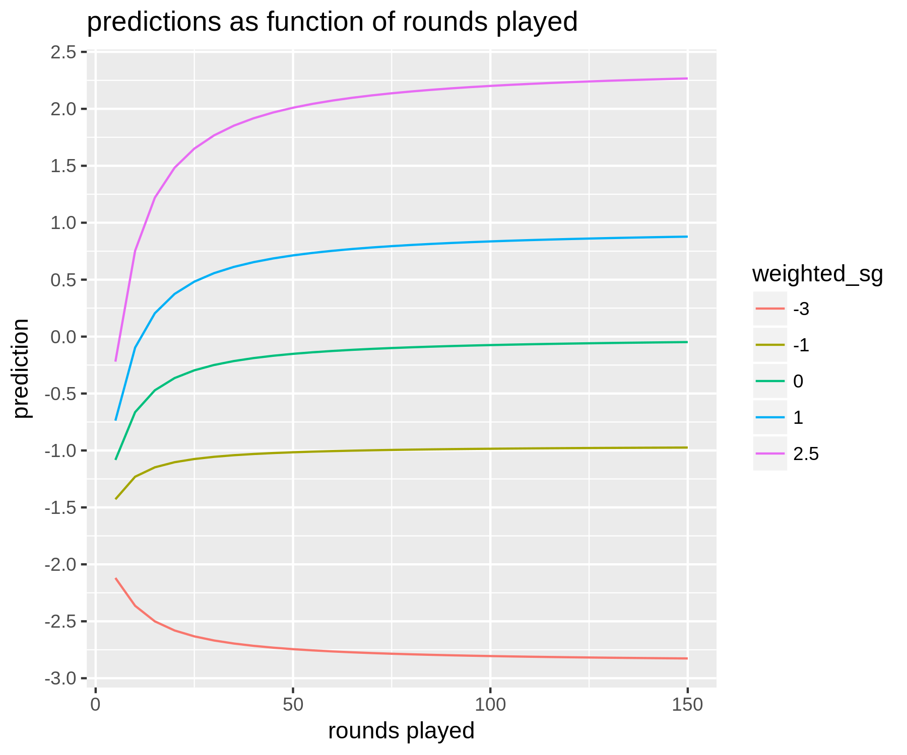
Notes: Plotted are predicted values from a regression model. Predictions (in units of SG per round) are a function of how many rounds a golfer
has played and their historical weighted average strokes-gained. The weighting scheme used here to construct the weighted average would be considered middle of
the road in terms of how heavily it weights recent versus older rounds. All predictions are
are for a golfer who played in the previous week.
There are a couple main takeaways here. First, even for golfers who have played a lot
(i.e. 150 rounds or more), there is some regression to the mean. That is,
if a golfer has a weighted average of +2 then our prediction for their next
tournament-round might be just +1.8.
Importantly, how much regression to the mean is present depends on
the weighting scheme. Longer-term weighting schemes (i.e. those that don't weight recent
rounds that much more than less recent ones) exhibit less regression to the mean, while shorter-term weighting schemes
exhibit more. This makes sense intuitively, as we would expect short-term
form to be less predictive than long-term form. However, what might be a little
less intuitive is the fact that these shorter-term weighting schemes can
outperform the longer-term ones. The reason is that although short-term
form is not as predictive as long-term form — in the sense that a 1 stroke increase in scoring average
over a shorter time horizon does not translate to an average increase in 1 stroke moving
forward, while a 1 stroke increase in long-term form more or less does — there is more
variance in short-term form across players
[5].
The second takeaway is the pattern of discounting as a function of the number of rounds played.
As you would expect, the smaller
the sample of rounds we have at our disposal, the more a golfer's past performance
is regressed to the mean. As the number of rounds goes to zero, our predictions converge
towards about -2 adjusted strokes-gained. It should also be pointed out that another input
to the model is which tour (PGA, Euro, or Web.com) the tournament is a part of: this has an impact
on very low-data predictions, as rookies / new players are generally of different quality on different tours.
The predicted values from this regression are our estimates for the player-specific means. What about player-specific variances? These are estimated by analyzing the residuals from the regression model above. The residuals are used because we want to estimate the part of the variance in a golfer's adjusted scores that is not due to their ability changing over time. We won't cover the details of estimating player-specific variances, but will make general two points. First, golfers for whom we have a lot of data have their variance parameter estimated just using their data, while golfers with less data available have their variance parameters estimated by looking at similar golfers. Second, estimates of variance are not that predictive (i.e. high-variance players in 2017 will tend to have lower variances in 2018). Therefore, we regress our variance estimates towards the tour average (e.g. a golfer who had a standard deviation of 3.0 in 2018 might be given an estimate of 2.88 moving forward).
With an assumption of normality, along with estimates (or, predictions) of each golfer's mean adjusted strokes-gained and the variance in their adjusted strokes-gained, we can now easily simulate a golf tournament. Each iteration draws a score from each golfer's probability distribution, and through many iterations we can define the probability of some event (e.g. golfer A winning) as the number of times it occured divided by the number of iterations. (As indicated earlier, in practice we do not actually assume scores are normally distributed — although we do still use the player-specific variance parameters to inform the shape of the distributions we use for simulation.)
Incorporating detailed strokes-gained categories
The model above is fairly simple (which is a good thing).
But, given that total strokes-gained can be broken down into 4 categories, each of which
is (very conveniently) expressed in units of strokes per round, a logical next step
is to make use of this breakdown when attempting to predict total strokes-gained.
This will improve predictions if certain categories are more predictive
than others. For example, if strokes-gained off-the-tee (SG:OTT) is very predictive
of future SG:OTT, while strokes-gained putting (SG:PUTT) is not that predictive
of future SG:PUTT, then we should have different predictions for two players
who have both been averaging +2 total strokes-gained, but have achieved this
differently. More specifically, we would tend to predict that the golfer who
has gained the majority of those 2 strokes from his off-the-tee play to
stay near +2, while a golfer who gained the majority of their strokes through putting
would be predicted to move away from +2 (i.e. regress towards the mean).
Because of the fact that total strokes-gained equals the sum of its parts
(off-the-tee (OTT), approach (APP), around-the-green (ARG), and putting (PUTT)),
we can do some nice regression exercises. Consider the following regression:
$$ \normalsize (2) \>\>\>\>\>\>\>\>TOTAL_{ij} = \beta_{1}\cdot OTT_{i,-j} + \beta_{2} \cdot APP_{i,-j} + \beta_{3} \cdot ARG_{i,-j} + \beta_{4} \cdot PUTT_{i,-j} + u_{ij} $$
where \( \normalsize TOTAL_{ij} \) is total adjusted strokes-gained for player i in tournament-round
j, and the 4 regressors are all defined similarly as some weighted average for
each category using all rounds up to but not including round j [6]. Therefore,
in this regression we are predicting total strokes-gained using a golfer's historical averages
in each category (all of which are adjusted [7]). We can also run 4 other regressions where we replace the dependent variable
here \( \normalsize (TOTAL_{ij} \)) with the golfer's performance in round j in each strokes-gained category (OTT, APP, etc.). This will have the nice property
that the 4 coefficients on \( \normalsize OTT_{i, -j} \) (for example) from the latter 4 regressions will add
up to \( \normalsize \beta_{1} \) in the regression above.
So what do we find? The coefficients are, roughly, \( \normalsize \beta_{1} = 1.2 \), \( \normalsize \beta_{2} = 1 \),
\( \normalsize \beta_{3} = 0.9 \), and \( \normalsize \beta_{4} = 0.6 \). Recall their interpretation: \( \normalsize \beta_{1} \) can be thought of
as the predicted increase in total strokes-gained from having a historical average SG:OTT that is 1 stroke higher,
holding constant the golfer's historical performance in all other SG categories. Therefore, the fact that
\( \normalsize \beta_{1} \) is greater than 1 is very interesting (or, worriesome?!). Why would a 1 stroke increase in
historical SG:OTT be associated with a greater than 1 stroke increase in future total strokes-gained? We can
get an answer by looking at our subregressions: using \( \normalsize OTT_{ij} \) as the dependent variable, the coefficient
is close to 1 (as we would perhaps expect), using \( \normalsize APP_{ij} \) the coefficient is 0.2, and for the other two categories
the coefficients are both roughly 0. So, if you take these estimates seriously (which we do; this is a robust result),
this means that historical SG:OTT performance has predictive power not only for future SG:OTT performance, but also
for future SG:APP performance. That is interesting. This means that for a golfer who is currently averaging
+1 SG:OTT and 0 SG:APP, we should predict their future SG:APP to be something like +0.2. A possible story here is that
a golfer's off-the-tee play provides some signal about a golfer's general ball-striking ability (which we would
define as being useful for both OTT and APP performance). The other coefficients
fall in line with our intution: putting is the least predictive of future performance.
How can we incorporate this knowledge into our predictive model to improve it's performance? The main takeaways from the work above is that the strokes-gained categories differ in their predictive power for future strokes-gained performance (with OTT > APP > ARG > PUTT). However, a difficult practical issue is that we only have data on detailed strokes-gained performance for a subset of our data: namely PGA Tour events that have ShotLink set up on-site. We incorporate our findings above by using a reweighting method for each round that has detailed strokes-gained data available; if the SG categories aren't available, we simply use total strokes-gained. In this reweighting method, if there were two rounds that both were measured as +2 total strokes-gained, with one mainly due to off-the-tee play while the other was mainly due to putting, the former would be increased while the latter would be decreased. To determine which weighting works best, we just evaluate out-of-sample fit (discussed below). That's why prediction is relatively easy, while casual inference is hard.
How can we incorporate this knowledge into our predictive model to improve it's performance? The main takeaways from the work above is that the strokes-gained categories differ in their predictive power for future strokes-gained performance (with OTT > APP > ARG > PUTT). However, a difficult practical issue is that we only have data on detailed strokes-gained performance for a subset of our data: namely PGA Tour events that have ShotLink set up on-site. We incorporate our findings above by using a reweighting method for each round that has detailed strokes-gained data available; if the SG categories aren't available, we simply use total strokes-gained. In this reweighting method, if there were two rounds that both were measured as +2 total strokes-gained, with one mainly due to off-the-tee play while the other was mainly due to putting, the former would be increased while the latter would be decreased. To determine which weighting works best, we just evaluate out-of-sample fit (discussed below). That's why prediction is relatively easy, while casual inference is hard.
Incorporating course fit (or not?)
We have argued in the
past that there is no statistically responsible way to incorporate
course history into a predictive model. But, after watching the Americans get slaughtered
at the 2018 Ryder Cup at Le Golf National in France, we came away thinking that course
fit was something we had to try to incorporate into our models. Spoiler alert: we tried
two approaches, and failed. In the first
approach, we tried to correlate a golfer's historical strokes-gained performance in the different categories (OTT, APP, etc.)
with that golfer's performance at a specific course. The logic here is that perhaps
certain courses favor players who are good drivers of the ball (i.e. good SG:OTT [8]), while other courses
favour players who are better around the greens (i.e. good SG:ARG). For some courses we have a reasonable
amount of data (e.g. 9 years worth for events that have been hosted on the same course
since 2010). The problem is that, even for these relatively high data courses,
the results are still very noisy.
It is true that
if you run the regression as in (2) separately for each course in the data,
you will find results that are different (to a *statistically significant* degree) from
the baseline result in (2). For example, instead of SG:APP having a coefficient of 1,
for some courses we will find it has a coefficient of 0.5. Should we take these estimates
at face value? No, I don't think so. Statistical significance is not very meaningful
at the best of times, and especially not when you are running many regressions:
of course you will find some statistically significant
differences if you have 30 courses in your data and 4 variables per regression. The ultimate
proof is in whether this additional information improves your out-of-sample predictive
performance, and in our case it did not.
Our second attempt at incorporating course fit involved trying to group courses
together that have similar characteristics, and then essentially doing a course history
exercise except using a golfer's historical performance on the group of similar courses instead of just
a single course. We have done
this exercise before using course groupings based off course length.
This time we tried grouping courses using clustering algorithms,
where the main characteristics again involved the detailed strokes-gained categories (e.g. the % of variance
in total scores that was explained by each category).
Ultimately I do think this is the way to go if you want to
incorporate course fit: if you had detailed course data (perhaps about average fairway width,
length, etc.) you could potentially make more natural groupings than we did. Unfortunately in our
case, with the course variables we used, it was again mostly a noise mine. This has left us thinking that
there is not an effective way to systematically incorporate course fit into
our statistical models. The sample sizes are too small, and the measures of
course similarity to crude, to make much headway on this problem. That's not to say
that course history doesn't exist; it probably does. But to separate the signal
from the noise is very hard.
Model evaluation and selection
Given the analysis and discussion so far, we can now think of having a set of models to choose from
where differences between models are defined by a few parameters. These parameters are
the choice of weighting scheme on the historical strokes-gained averages (this involves just a single parameter that determines the rate of exponential decay
moving backwards in time), and also the weights that are used to incorporate the detailed strokes-gained
categories through a reweighting method.
The optimal set of parameters are selected through brute force: we loop through all possible combinations of parameters,
and for each set of parameters we evaluate the model's performance through a cross validation exercise.
This is done to avoid overfitting: that is, choosing a model that fits the estimating data very well but does not
generalize well to new data. The basic idea is to divide your data into a "training" set
and a "testing" set. The training set is used to estimate the parameters of your model (for our model,
this is basically just a set of regression coefficients [9]),
and then the testing set is used to evaluate the predictions
of the model. We evaluate the models using mean-squared prediction error, which in this context is defined as
the difference between our predicted strokes-gained and the observed strokes-gained, squared and then averaged.
Cross validation involves repeating this process several times (i.e. dividing your sample into training and
testing sets) and averaging the model's performance on the testing sets.
This repetitive process is again done to avoid overfitting. The model that performs the best in the cross validation
exercise should (hopefully) be the one that generalizes the best to new data. That is, after all, the goal of
our predictive model: to make predictions for tournament outcomes that have not occurred yet.
One thing that becomes clear when testing different parameterizations is how similar they perform overall
despite disagreeing in their predictions quite often.
This is troubling if you plan to use your model
to bet on golf. For example, suppose you and I both have models that
perform pretty similar overall (i.e. have similar mean-squared prediction error), but also
disagree a fair bit on specific predictions. This means that both of our models would find what
we perceive to be "value" in betting on some outcome against the other's model. However, in reality,
there is not as much value as you think: roughly half of those discrepancies will be cases
where your model is "incorrect" (because we know, overall, that the two models fit the data similarly).
This is not exactly a deep insight: it simply means that to assume your model's odds
as *truth* is an unrealistic best-case scenario for calculating expected profits.
The model that we select through the cross validation exercise has a weighting scheme that I would classify as "medium-term": rounds played 2-3 years ago do receive non-zero weight, but the rate of decay is fairly quick. Compared to our previous models this version responds more to a golfer's recent form. In terms of incorporating the detailed strokes-gained categories, past performance that has been driven more by ball-striking, rather than by short-game and putting, will tend to have less regression to the mean in the predictions of future performance.
The model that we select through the cross validation exercise has a weighting scheme that I would classify as "medium-term": rounds played 2-3 years ago do receive non-zero weight, but the rate of decay is fairly quick. Compared to our previous models this version responds more to a golfer's recent form. In terms of incorporating the detailed strokes-gained categories, past performance that has been driven more by ball-striking, rather than by short-game and putting, will tend to have less regression to the mean in the predictions of future performance.
Adapting model for live predictions
To use the output of this model — our pre-tournament estimates of the mean and variance
parameters that define
each golfer's scoring distribution — to make live predictions as a golf
tournament progresses, there are a few challenges to be addressed.
First, we need to convert our round-level scoring estimates to hole-level scoring estimates. This is accomplished using an approximation which takes as input our estimates of a golfer's round-level mean and variance and gives as output the probability of making each score type on a given hole (i.e. birdie, par, bogey, etc.).
First, we need to convert our round-level scoring estimates to hole-level scoring estimates. This is accomplished using an approximation which takes as input our estimates of a golfer's round-level mean and variance and gives as output the probability of making each score type on a given hole (i.e. birdie, par, bogey, etc.).
Second, we need to take into account the course conditions for each golfer's
remaining holes. For this we track the field scoring averages
on each hole during the tournament, weighting recent scores
more heavily so that the model can adjust quickly to
changing course difficulty during the round. (Of course, there is a tradeoff here
between sample size and the model's speed of adjustment.) Another important detail in
a live model is
allowing for uncertainty in future course conditions. This matters mostly
for estimating cutline probabilities accurately, but does also matter for
estimating finish probabilities. If a golfer has 10 holes
remaining, we allow for the possibility that these remaining 10 holes
play harder or easier than they have played so far (due to wind picking up
or settling down, for example). We incorporate this uncertainty
by specifying a normal distribution for each hole's future scoring average, with
a mean equal to it's scoring average so far, and a
variance that is calibrated from historical data [10].
The third challenge is updating
our estimates of player ability as the tournament progresses. This can be
important for the golfers that we had very little data on pre-tournament.
For example, if for a specific golfer we only have 3 rounds to make
the pre-tournament prediction, then by the fourth round of the tournament
we will have doubled our data on this golfer! Updating the estimate
of this golfer's ability seems necessary. To do this, we have a rough model
that takes 4 inputs: a player's pre-tournament prediction, the number of
rounds that this prediction was based off of, their performance
so far in the tournament (relative to the appropriate benchmark),
and the number of holes played so far in the tournament. The predictions
for golfers with
a large sample size of rounds pre-tournament will not be adjusted very
much: a 1 stroke per round increase in performance during the tournament translates
to a 0.02-0.03 stroke increase in their ability estimate (in units of
strokes per round). However, for a very low data player, the ability update could be
much more substantial (1 stroke per round improvement could translate to 0.2-0.3 stroke updated ability
increase).
With these adjustments made, all of the live probabilities of interest can be estimated through simulation. For this simulation, in each iteration we first draw from the course difficulty distribution to obtain the difficulty of each remaining hole, and then we draw scores from each golfer's scoring distribution taking into account the hole difficulty.
With these adjustments made, all of the live probabilities of interest can be estimated through simulation. For this simulation, in each iteration we first draw from the course difficulty distribution to obtain the difficulty of each remaining hole, and then we draw scores from each golfer's scoring distribution taking into account the hole difficulty.
Changes to the model for 2020
The clear deficiency in earlier versions of our model was that no course-specific
elements were taken into account. That is, a given golfer had the same predicted mean (i.e. skill) and
variance regardless of the course they were playing.
After spending a few months slumped over our computers, we can now happily
say that our model incorporates both course fit and course history for PGA Tour events.
(For European Tour events, the model only includes course history adjustments.)
Further, we now account for differences in course-specific variance, which captures
the fact that some courses have more unexplained variance (e.g. TPC Sawgrass) than others (e.g. Kapalua).
This will be a fairly high-level explainer. We'll tackle course fit and then course-specific variance in turn. The approach to course fit that was ultimately successful for us was, ironically, the one we described in a negative light a year ago. For each PGA Tour course in our data we estimate the degree to which golfers with certain attributes under or over-perform relative to their baselines (where a golfer's baseline is their predicted skill level at a neutral course). The attributes used are driving distance, driving accuracy, strokes-gained approach, strokes-gained around-the-green, and strokes-gained putting. More concretely, we correlate a golfer's performance (i.e. strokes-gained) at a specific course with an estimate of their skill level in each attribute (distance, accuracy, approach, etc.) at that point in time. Attribute-specific skill levels are obtained using analogous methods to those which were described in an earlier section to obtain golfers' overall skill level. For example, a player's predicted driving distance skill at time t is equal to a weighted average of previous adjusted (for field strength) driving distance performances, with more recent rounds receiving more weight, and regressed appropriately depending on how many rounds comprise the average. The specific weighting scheme differs by characteristic; not suprisingly, past driving distance and accuracy are very predictive of future distance and accuracy, and consequently relatively few rounds are required to precisely estimate these skills. Conversely, putting performance is much less predictive, which results in a longer-term weighting scheme and stronger regression to the mean for small samples.
With estimates of golfer-specific attributes in hand, we can now attempt to estimate a course-specific effect for each attribute on performance — for example, the effect of driving distance on performance (relative to baseline) at Bethpage Black. The main problem when attempting to estimate course-specific parameters is overfitting. Despite what certain sections of Golf Twitter would have you believe, attempting to decipher meaningful course fit insights from a single year of data at a course is truly a hopeless exercise. This is true despite the fact that a year's worth of data from a full-field event yields a nominally large sample size of roughly 450 rounds. Performance in golf is mostly noise, so to find a predictive signal requires, at a minimum, big sample sizes (it also requires that your theory makes some sense). To avoid overfitting, we fit a statistical model known as a random effects model. It's possible to understand its benefits without going into the details. Consider estimating the effect of our 5 attributes on performance-to-baseline separately for each course: it's easy to imagine that you might obtain some extreme results due to small sample sizes. Conversely, you could estimate the effect of our 5 golfer attributes on performance-to-baseline by pooling all of the data together: this would be silly as it would just give you an estimate of 0 for all attributes (as we are analyzing performance relative to each golfer's baseline, which has a mean of zero, by definition). The random effects model strikes a happy medium between these two extremes by shrinking the course-specific estimates towards the overall mean estimate, which in this case is 0. This shrinkage will be larger at courses for which we have very little data, effectively keeping their estimates very close to zero unless an extreme pattern is present in the course-specific data. Here is a nice interactive graphic and explainer if you want more intuition on the random effects model. Switching to this class of model is one of the main reasons our course fit efforts were more successful this time around.
What are the practical effects of incorporating course fit? While in general the difference between the new model, which includes both course fit and course history adjustments, and the previous one (which we'll refer to as the baseline model) are small, there are meaningful differences in many instances. If we consider the differences between the two models in terms of their respective estimated skill levels (i.e. the player-specific means), the 25th and 75th percentiles are -0.07 and +0.07 respectively, while the minimum and maximum are -0.93 and +0.95, respectively (units are strokes per round). I can't say I ever thought there would come a day when we would advocate for a 1 stroke adjustment due to course fit! And yet, here we are. Let's look at an example: before the 2011 Mayakoba Classic at El Camaleon Golf Club, we estimated Brian Gay to be 21 yards shorter off the tee and 11 percentage points more accurate (in fairways hit per round) than the PGA Tour average. This made Gay an outlier in both skills, sitting at more than 2 standard deviations away from the tour mean. Furthermore, El Camaleon is probably the biggest outlier course on the PGA Tour, with a player's driving accuracy having almost twice as much predictive power on performance as their driving distance (there are only 11 courses in our data where driving accuracy has more predictive power than distance). Therefore, at El Camaleon, Gay's greatest skill (accuracy) is much more important to predicting performance than his greatest weakness (distance). Further, Gay had had good course history at El Camaleon, averaging 1.2 strokes above baseline in his 12 previous rounds there. (It's worth pointing out that we estimate the effects of course history and course fit together, to avoid 'double counting'. That is, good course fit will often explain some of a golfer's good course history.) Taken together, this resulted in an upward adjustment of 0.9 strokes per round to Gay's predicted skill level for the 2011 Mayakoba Classic.
When evaluating the performance of this new model relative to the baseline model, it was useful to focus our attention on observations where the two models exhibit large discrepancies. The correlation between the two models' predicted skill levels in the full sample is still 0.99; as a consequence the difference between their respective prediction errors using the full sample will always be relatively small. However, by focusing on observations where the two models diverge substantially, it becomes clear that the new model is outperforming the baseline model.
As previously alluded to, the second course-specific adjustment we've made to our model is the inclusion of course-specific variance terms. This means that the player-specific variances will all be increased by some amount at certain courses and decreased at others. It's important to note that we are concerned with the variance of 'residual' scores here, which are the deviations in players' actual scores from our model predictions (this is necessary to account for the fact that some courses, like Augusta National, have a higher variance in total scores in part because there is greater variance in the predicted skill levels of the players there). All else equal, adding more unexplained variance — noise — to scores will bring the model's predicted win probabilities (for the tournament, for player-specific matchups, etc.) closer together. That is, Dustin Johnson's win probability at a high (residual)-variance course will be lower than it is at a low-variance course, against the same field. In estimating course-specific variances, care is again taken to ensure we are not overfitting. Perhaps surprisingly, course-specific variances are quite predictive year-over-year, leading to some meaningful differences in our final course-specific variance estimates. Examples of some of the lowest variance courses are Kapalua, Torrey Pines (North), and Sea Island (Seaside); some of the highest variance courses are Muirfield Village, TPC Sawgrass, and Whistling Straights. A subtle point to note here is that a course can simultaneously have high residual variance and also be a course that creates greater separation amongst players' predicted skill levels. For example, at Augusta National, golfers with above-average driving distance, who tend to have higher baseline skill levels, are expected to perform above their baselines; additionally, Augusta National is a course with above-average residual variance. Therefore, whether we would see the distribution of win probabilities narrow or widen at Augusta (relative to a typical PGA Tour course) will depend on which of these effects dominates.
Changes to the model for 2021
There are a few important changes to the 2021 model. First, we are now incorporating
a time dimension to our historical strokes-gained weighting scheme. This was an important missing element
from earlier versions of the model. For example, when Graham DeLaet returned in early 2020 after a
1-year hiatus from competitive golf, our predictions were mostly driven by his data
from 2018 and earlier, even after DeLaet had played a few rounds in 2020. It seems intuitive that more weight
should be placed on DeLaet's few rounds from 2020 given the absence of 2019 data (compared to a scenario where he had played a full
2019 season). Using a weighting function that decays with time (e.g. days) achieves this. However,
continuing with the DeLaet example, there is still lots of information contained in his pre-2019
rounds. Therefore we use an average of our two weighted averages: the first weights rounds by the sequence
in which they were played, ignoring the time between rounds, while the second assigns weights based
on how recently the round was played. In DeLaet's case, if he were playing this week (Jan 4, 2021), his time-weighted predicted
strokes-gained would be -3.1, while his sequence-weighted predicted strokes-gained
would be -1.1. Ultimately we combine these two predictions and end up with a final prediction of -2.5 (we don't just take a
simple average of the two; it depends on a couple parameters). The difference between this value
and the sequence-weighted average is what appears in the "timing" column on the
skill decomposition page. Have a look
at DeLaet's true strokes-gained plot to understand why the different weighting methods cause such a large divergence
in estimated skill. For golfers who are playing a steady schedule, there will not be large differences
between the time-weighted and sequence-weighted strokes-gained averages. However for players that play an above-average
number of rounds per year (e.g. Sungjae Im), the time-weighting will tend to de-emphasize their most recent data.
A second change to the 2021 model is that we are using yet another method to incorporate the strokes-gained categories into our baseline (i.e. pre-course fit / history) predictions. As we've said elsewhere, it is surprisingly difficult to use the strokes-gained categories in a way that doesn't make your predictions worse. This is because not all PGA Tour and European Tour events have strokes-gained data (which reminds me: another new thing for this season is that we have added European Tour SG category data). Therefore, if you were to leverage the category SG data but (necessarily) only use rounds with detailed SG data, you would be outperformed by a model that only uses total strokes-gained but uses data from all events. This highlights the importance of recent data in predicting golf performance. Our previous strokes-gained category adjustment method involved predicting performance in the SG categories using total SG in rounds where the categories weren't available, and then estimating skill in each SG category using a combination of the real and imputed SG data. This worked reasonably well but had its drawbacks. I'll omit the details on our current method, but it no longer uses imputed SG data. The general goal when incorporating the SG categories is to account for the fact that estimating skill in ARG / PUTT requires a larger sample size than does APP / OTT. Therefore, if a golfer's recent performance is driven by a short-term change in ARG or PUTT, their SG adjustment will be in the opposite direction of that recent change (e.g. a short-term uptick in putting performance from a golfer's long-term baseline results in a negative SG category adjustment). The logic is reversed for OTT: if the recent uptick in performance is driven by OTT play, the SG category adjustment will be positive.
A third model update involves how our predictions are updated between rounds within a tournament. In the past we have been a bit lazy when predicting a golfer's Round 2 (R2) performance given their R1 performance (plus historical pre-tournament data). Now we have explicity estimated what that update should be, and, interestingly, we also allow the weight applied to a golfer's R1 performance to vary depending on a few factors. These factors include the number of days since a golfer last played an event (this increases the weight on R1 performance when predicting R2, all else equal), the total number of rounds a golfer has played (this really only matters for players with fewer than ~50 rounds), and also a measure of the overall recency of a player's data. For example, as mentioned above Sungjae Im is a golfer who doesn't take many weeks off; therefore, when predicting his R2 performance, Im's R1 score is weighted less than the typical tour player. It should be clear that this is tightly linked to the ideas behind using a time-weighted decay; the further into the past is the bulk of a golfer's historical data, the more weight their R1 performance will receive when predicting R2. Similar logic is applied when predicting R3 and R4 performance. This will have obvious implications for our model when predicting performance after a tournament starts (e.g. for the live model, R2 matchups), but it also matters for pre-tournament predictions. The stronger the correlation between within-tournament performances (e.g. the larger the weight on R1 when predicting R2), the larger is the variance in a golfer's tournament outcomes. Thinking through the simulation of a golf tournament can help clarify this: if a golfer plays well in the first round their predicted skill for the second round simulation is increased, while if they play poorly their R2 skill is decreased. The larger the weight on R1 performance, the wider is the range of their possible predicted skill levels for R2, which in turn leads to a wider range of potential scores. Compared to our previous model, this change in within-tournament weighting does not make a huge difference for pre-tournament predictions, but it will be noticeably different once the tournament starts and skill levels are actually updated. I'm also excited about how the differential weighting can handle players coming off of long layoffs, as I've always felt these golfers' skill estimates should respond more to their R1/R2/R3 performances. A final point is that we also incorporate the strokes-gained categories into the within-tournament updates when possible (leveraging the fact that, eg, outperforming one's baseline in OTT in R1 is much more informative than doing the same with putting).
Finally, the European Tour version of our model in 2021 will now include course fit adjustments. Course fit, along with the aforementioned addition of European Tour strokes-gained category data, should bring the quality of our Euro predictions up to the level of our PGA predictions.
Recent model happenings (mid-2021 update)
There have been enough changes in our model recently to warrant a deviation from our previous schedule of once-a-year
written updates. We also think it's important for our users, as we try to add model customizability
to the site, to know what our model is taking into
account in order to understand the dimensions along which it can be improved.
Therefore this is partly an attempt to put more relevant information about our model in one place.
Now, to the updates.
First — and this was actually added sometime in late 2020 — the effects of "pressure" are now included in the model. This is an adjustment we make to players' predicted skill in the third and fourth rounds that depends on their position on the leaderboard to start the day. This is not a player-specific adjustment, and does not vary depending on player characteristics either (e.g. elite vs. non-elite golfers). We haven't found meaningful differences in performance relative to expectation when leading across categories of players — it seems everyone performs worse when near the lead. There are a lot more details on the pressure-performance relationship in this blog and on this interactive page.
Second, we recently revisited the question of the optimal decay rates for the various weighting schemes used on a player's historical data. Relative to the market it seems like our model weights longer-term data more heavily. For some context, when using only total strokes-gained to predict future performance, our model places about 70% of the weight on the most recent 50 rounds for a golfer who has been playing a full schedule. This is for the sequence-weighted average described in the section above this one. Also mentioned in that section, and this was a new addition for 2021, was the time-weighted average. We have now made that weighting scheme slightly more short-term oriented. The interesting, general, thing that we learned by revisiting these decay rates is that the optimal weighting scheme for a specific weighted average shouldn't be chosen in isolation. For example, if we were only to use a sequence-weighted average to predict performance, then the optimal decay would be larger (i.e. more weight on the short-term) than if we use it in conjunction with a time-weighted average. In this specific case, I think that makes sense, as the role of the sequence-weighted average is in part to pick up longer trends in performance if a player hasn't played much recently.
The other weighting schemes we revisited are those used on the specific strokes-gained categories. Omitting the details, we are also now slightly more short-term focused on all the SG categories (for the same reason specified above — when using the categories together instead of in isolation, it appears that short-term weighting schemes are slightly better). The upshot of this is that the strokes-gained category adjustments used to be somewhat biased towards longer-term data. That is, even ignoring differential performance in the categories, which is what we want to be driving that adjustment, if a player was performing well in the short-term they were likely to be receiving a negative SG adjustment. Going forward this will no longer be an issue. While on the topic of the SG adjustment, it's worth mentioning the European Tour SG category data. As discussed here, because most of the Euro SG category data are event-level averages we have to impute the round-level values. This is not a huge issue, but it does make it difficult to actually fit a model for predicting strokes-gained categories at the round level on the European Tour. As a result, we have to rely on our PGA Tour models for the SG categories and hope the relationships in that data also hold in the Euro data. The degree to which this works can still ultimately be tested by looking at whether our overall predictions are improved. However, again there are issues: we only have 4 years of European tour strokes-gained category data, which is not quite enough to get precise answers. We want to determine if we can use the European SG category data in some way to improve over our baseline predictions which are based off only total SG data; these two estimates of skill will inevitably be very highly correlated, and so over 4 years there actually aren't that many instances where the two methods will disagree substantially (allowing for their respective predictive performance to be compared). In any case, the practical takeway here is that we are decreasing the size of the SG category adjustments we make on the European Tour slightly.
With regards to the overall long-term versus short-term focus of our model, it is useful to consider two recent examples of players that we didn't update as quickly on relative to the market: Jordan Spieth and Lee Westwood. They are instructive examples of cases that our model might not handle well for different reasons. In the case of Spieth, part of the reason the market reacted so quickly was that Spieth had proven himself to be a world-beater early in his career. The idea seemed to be that once Spieth flashed some of his old form we could essentially ignore the data from the two-year slump he was pulling himself out of. While I obviously don't agree with ignoring the slumping-Spieth data, I do think it's important to account for the fact that Spieth used to be a top player; our current model doesn't do this, as rounds from more than a couple years ago essentially receive no weight. We are working on a few different ideas to handle these cases, but it's a tricky problem to find a systematic solution to. In the case of Lee Westwood, I think the reason the market adjusted so quickly was that he had two massive outlier performances (gaining around 4, and then 3.5, strokes above expectation in back-to-back events). Westwood's performances at the API and The Players were his 1st and 3rd largest positive deviations from our model's expectation since 2015. I think a case could be made for making proportionally larger adjustments for larger deviations from expectation (e.g. adjust more than 2x when a player gains 4 strokes versus 2 strokes). Using some form of Bayesian updating, which uses the likelihood of something occuring to inform the size of the update, might achieve this but it's not clear how we would go about it. However it's also important to remember that while it was unlikely for Westwood specifically to have back-to-back outlier weeks like he did, it was not that unlikely that someone would do it. Just like it's exceedingly unlikely for a specific person to win the lottery, but someone has to win it. Given how Westwood has performed since those 2 weeks, it seems like there hasn't been an actual shift in his skill level; Spieth, on the other hand, appears to be back.
Third, it's worth going into a little more detail on the within-tournament updates to player skill levels. We haven't changed anything in our approach since the start of 2021, but it is interesting and we skimmed over it in the previous section. Compared to previous versions of our model, a player's skill level now has the potential to be updated much more as a result of their performance during a tournament. For example, performing 1 stroke above expectation off the tee in round 1 leads to a 0.12 stroke update in projected skill for round 2. (In all of this, there are several adjustments made to ensure that each golfer's strokes-gained category skill estimates add up to our estimate of what their overall skill is. This adjustment can be large if most of a player's data is from events without detailed SG data.) Deviations from expected performance in the other SG categories carry considerably less predictive weight (with APP > ARG ~ PUTT), however there are also greater deviations from expectation in approach and putting performance than those seen off the tee. I think the reason off-the-tee performance in a single round can be so predictive is partly just because it is a lower-noise statistic, but also because it provides the most information about course fit. Driving distance and driving accuracy show the largest differences across courses in their course-specific predictive power; assuming these effects operate mainly through off-the-tee play (although it likely happens through approach as well), it's reasonable to think that first round performance is providing some information on the golfer's course fit (that we haven't captured in our pre-tournament fit adjustments). This information still comes with a lot of noise, but it does add to the signal we can glean from that single round. When strokes-gained category data is not available we only update skill levels based off of total strokes-gained.
Fourth, weather is now explicity accounted for in the model. We mainly focus on wind forecasts, as the effect of wind on performance is the most straightforward to predict (whereas rain could make a course play easier or harder, depending on the specific course setup). In our pre-tournament simulations each player receives an adjustment to their expected strokes-gained per round based on the projected wind conditions for the time window that they'll be on the course. Simple enough. In our live simulations, we have to use both historical and forecasted weather conditions to predict how the remaining holes will play for each golfer. The historical part is necessary because it's not enough to know, for example, that Brian Harman is expected to face a 10mph wind over his next 9 holes; we also need to know the weather conditions from earlier in the day that led to the current scoring average on those holes. Our approach is to first adjust our historical scoring data to a set of baseline conditions (e.g. 5mph wind). This includes data from past years, rounds, waves, and of course the scoring data from earlier in the day. We then use pre-fit models that take as inputs all data from before the current wave of golfers. Then, we use an explicitly Bayesian update to combine this start-of-wave prediction with the live scoring data from that wave. This is easy to do if we assume our start-of-wave projection is normally distributed and also that golf scores are normal. The result is a live estimate of each hole's difficulty under the baseline weather conditions which, given the normality assumption, is encapsulated in a mean (i.e. the expected scoring average for the hole) and a variance (i.e. the uncertainty around this expectation). Returning to the Harman example, all that is left is to make a scoring adjustment (e.g. 0.05 strokes per 1mph of wind) that accounts for the difference between Harman's forecasted conditions and baseline conditions. (For some intuition on thinking through how this fits into a simulation, see this FAQ section.) The final piece of this puzzle was added very recently, and that was factoring in player skill when estimating course difficulty. Just as with weather, we can adjust the observed scoring averages for each hole to reflect what we would expect from some baseline golfer; then, to project Brian Harman's performance, we simply add in an adjustment to account for the difference between Harman's skill and that of our baseline golfer. (Previously, we would assume that observed scoring averages came from a group of players with an average skill level equal to the field's average — which, is generally an OK assumption except when there are only a few players on the course.) The impact of these changes to the live model are most noticeable when projecting the cutline, but also matter for projecting any outcome of a golf tournament when the players involved have differing numbers of holes remaining or will be playing their remaining holes at different times. With these adjustments, our live model is now pretty good at projecting both the expected course conditions and the uncertainty around those conditions.
Fifth and finally, we are starting to incorporate shot-level information into the model. One simple adjustment we are currently making relates to hole outs: we decrease a player's strokes-gained in a given round by 1 stroke for every shot they hole out from a distance above some (arbitrarily chosen) threshold. The idea here is that it's completely luck whether or not a shot ends up an inch from the hole or in it, but the difference in strokes-gained between these two scenarios is a full stroke. The effect of these adjustments on golfers' predicted skill levels are small, rarely exceeding 0.05 strokes. For a little more detail on this, see the 4th number of this ITN.