Feb 9, 2021
The Favourite-Longshot Bias is not a bias
The so-called "favourite-longshot (FL) bias" is the well-documented observation from
betting markets that bets placed at higher offered odds (longshots) yield
worse rates of return than bets placed at lower odds (favourites).
This empirical regularity has received
attention from academics and intellectually-inclined gamblers for decades. It has been a
very robust finding: few betting markets have been studied that did not
exhibit lower rates of return at longer odds.
Why do academics, specifically economists, care so much about this pattern? The favourite-longshot bias has often been interpreted as a real-world example of irrational behaviour and market inefficiency. Indeed, we should ask, if the rate of return is worse on bets with longer odds, why do bettors take those bets? Why don't market forces, in the form of bettor demand, act on these offered prices until their rates of return are equal? Viewed through the lens of standard economics, the favourite-longshot pattern seemingly requires a non-standard explanation.
As its title suggests, the thesis put forward here is that the favourite-longshot bias is not a "bias"; it is not the result of bettor irrationality or non-standard preferences, nor is it an example of market inefficiency. We'll proceed as follows. The first section makes the intuitive case for the inevitability of lower rates of return at longer odds relative to returns at shorter odds. At very short odds, e.g. events that have "true", or objective, probabilities greater than 99%, a bookmaker can only apply so much margin without making the offered price absurd (i.e. exceeding 100%). A proportional allocation of the margin — which is required to equalize the rate of return across all offered bets — forces the bookmaker to reduce the total margin to keep the favourite's price below 100%, which in turn creates an essentially margin-free price on the longshot. Neither of these options — offering a price in excess of 100% on a favourite, or a margin-free price on the longshot — could possibly be optimal from the bookmaker's perspective, and yet one of them is required if all offered bets are to have equal expected returns. The second section highlights a simple but important point, and one that appears to have been overlooked: in research on this subject, the FL bias is defined differently in "traditional" gambling markets (e.g. bookmaker, parimutuel) from how it is defined in prediction markets. More specifically, in traditional betting markets the favourite-longshot bias is defined as I have introduced it here: worse rates of returns at longer odds. However, in prediction markets, researchers define the favourite-longshot bias as a scenario in which the midpoint of the bid-ask spread overestimates the objective outcome probability at longer odds. A small puzzle in the literature has been why the favourite-longshot bias seems to be less prevalent in prediction markets than traditional betting markets. The answer is simple: the absence of a bias in the midpoint of the bid-ask spread implies returns will decrease as odds lengthen. That is, the absence of an FL pattern using the prediction market definition implies there will be an FL pattern using the traditional definition. The one exception to this is a market where there are zero transcation costs (i.e. no margin in a bookmaker's odds, or no spread in the bid-ask); in this case the two definitions of the favourite-longshot bias are equivalent. While all of the traditional betting markets that have been empirically studied and shown to exhibit the FL bias have non-zero margin, many of the theoretical models used to explain the bias exclusively consider the special case of zero transaction costs. This is problematic. The third section presents a basic economic model of a betting market. Both the bookmaker and the bettors in this model are behaving rationally, but equilibrium offered odds will be such that worse returns for bettors are realized at longer odds. The only twist in this model is that bettors are heterogeneous: they disagree on the probability of the event occurring. I explain why the standard "representative bettor" model is not useful for describing a betting market, and argue that the model I present is the simplest and most intuitive description of how bettors and "sharp" bookmakers interact. The fourth section first analyzes data from soccer markets at a sharp bookmaker (Pinnacle). These are markets that see very high volume and have many sophisticated participants; I document the extent of the favourite-longshot bias and compare it to the predictions of the model presented in Section 3. I then take a closer look at the motivating empirical evidence from a well-known paper on the FL bias. The final section concludes.
Just give me the intuition
The market setup I use throughout this post is as follows.
All contracts have only two possible outcomes: they pay out 1 unit if the event occurs and 0 otherwise.
The market will be described
only by "win" contracts: for example, if we consider a two-golfer contest
between Golfer A and Golfer B,
the two contracts offered will be "Golfer A wins" and "Golfer B wins" (and not "Golfer A does not win",
"Golfer B does not win"). The price of these 1-unit-win contracts is the implied probability
of the contract — that is, the required probability for the contract to have an expected value of zero.
This formulation is essentially how traditional bookmaker markets are presented, except
instead of the payout being fixed at 1 unit, books list as odds the payout you receive
from a winning 1 unit bet.
For example, a bet with European
odds of 3.0 means you receive a payout of 3 units
on a 1 unit bet (for a profit of 2 units) if the event occurs; this is equivalent
to a 1-unit-win contract with a price of 1/3.
Conveniently, this formulation can be easily related to a prediction market
setting, with the added advantage that it is easy to calculate the expected rate of return on 1-unit-win contracts (in contrast
to a bid-ask or back-lay setup — both common in prediction markets — which makes
calculating rates of return less obvious, as
Section 2 highlights).
To understand why it would be very unusual for a betting market to not exhibit lower returns at longer odds, we'll look at a simple example. Consider a contest between Golfer A and Golfer B, where the true probability of Golfer A winning is 99% and the true probability of Golfer B winning is 1%. A bookmaker, or a market-maker in a prediction market, will create a market for this match such that they have an advantage. This advantage is built by offering a complete set of 1-unit-win contracts whose prices sum to greater than 1; the amount by which this sum exceeds 1 is called the bookmaker's margin. For expected returns to be equal on all contracts we require that this overall margin is allocated proportionally to each contract. For example, the bookmaker might offer a set of contracts that sum to 105%; proportional allocation of this margin would imply prices for the individual contracts of \( 0.99 \cdot 1.05 = 1.0395 \) and \( 0.01 \cdot 1.05 = 0.0105 \) for Golfer A and Golfer B, respectively. The expected returns on these contracts for a prospective bettor would be the same and equal to -4.76%. However the contract on Golfer A is, of course, absurd: you are guaranteed to lose money given that the payout if Golfer A wins is only 1 unit. An obvious objection to this example is the assumption of 5% total margin; if the bookmaker applies less total margin, then perhaps a proportional allocation does not make an absurd price. To keep the price for Golfer A below 1 with a proportional allocation requires that the total margin is no greater than 1.01%. This threshold seems reasonable enough, until we consider the price for Golfer B from a proportional allocation of this 1.01% margin: 0.010101. For readers who prefer odds notation, this is equivalent to European odds of 99 and American odds of +9800 (and the fair price of 0.01 is equivalent to 100 and +10000, respectively). As the true probability for Golfer A approaches 1, a proportional margin allocation requires that the bookmaker choose between offering a price in excess of 1 on the favourite or an essentially margin-free price on the longshot. It strains credulity to believe this could be optimal behaviour for a bookmaker, which begs the question: why should we expect the bookmaker's margin to be allocated proportionally?
One way to model a betting market is to assume that all bettors are identical, risk-neutral, utility-maximizing agents. Equivalently, in this model, we can think of there only being a single "representative" bettor, instead of many identical ones. The fact that the bettor is risk-neutral means she only cares about expected returns (and not the variance in returns). The only equilibrium that can be supported in this model is one where expected returns are equalized across all offered bets; if returns weren't equal, our representative bettor would put all her money on the higher expected value bet. This model provides a rationale for the proportional allocation of a bookmaker's margin, as it is the only allocation that equalizes the rate of return across bets. Under this model of the betting market, the empirical finding of lower returns at longer odds is viewed as a bias: how can our representative bettor be indifferent to all offered bets if the expected returns are not equal? The two most common early answers to this question were: 1) people who gamble are not risk-neutral, but risk-loving; this means they are willing to take lower expected value propositions for higher upside (and downside), and 2) people over-estimate small probabilities and under-estimate large probabilities, so they perceive expected returns to be equalized across longshots and favourites even though they aren't in reality. Much of economic theory is built on the assumption that people are risk-averse and rational (a loaded term, but for our purposes this means they can assess probabilities in an unbiased fashion); the favourite-longshot bias appears to fly in the face of this, which is why it has received a lot of attention.
It is an intriguing line of reasoning. However, modelling a betting market where there is non-zero margin added to the prices with a representative bettor does not make much sense. Under that setup, we immediately have the troubling question of why this bettor is participating in the market to begin with; if they are indifferent to all offered odds, and the odds sum to more than 100% (due to a bookmaker's margin), then the bettor knows she will lose money in the long run. To get around this, the misperceptions explanation (#2 above) requires an additional assumption to rationalize why the bettor participates in the market; it's common in the academic literature to assume that bettors receive some non-monetary utility from gambling that makes up for the negative expected return (e.g. entertainment value). While this could be true at lower stakes, it does not hold much water in high-volume markets like Pinnacle's soccer markets. The risk-love explanation (#1 above) is appealing in the sense that it also provides a rationale for participation in a negative expected value betting market; however it is unappealing for the obvious reason that it requires us to assume that people are willing to pay for more risk (when in most other contexts the opposite appears to be true). The bottom line is this: if you handcuff yourself to the assumption of identical bettors, then you are forcing these bettors to be either irrational (e.g. misestimate probabilities) or to have non-standard preferences (e.g. risk-loving) in order to explain the FL bias. However, if you relax the assumption of identical bettors (as models of prediction markets already do), the simplest model with rational bettors and a rational bookmaker predicts declining returns at longer odds. This model will be introduced and explored in the third section.
An important difference in definition
Lower expected returns at longer odds is how the favourite-longshot bias is typically defined
(see [1], [2]). In an otherwise excellent paper on
prediction markets by Justin Wolfers and
Eric Zitzewitz [3], they document the favourite-longshot bias from a traditional fixed odds
betting market for horse racing by examining rate of return as a function of
odds (p.12); however,
on the very next page they investigate whether a bias is present in a
prediction market by examining the midpoint
of the bid-ask spread, failing to notice that these two examples are not conveying the same information.
In the second example, there is in fact a very substantial and monotonic decline in the rate of return
as odds lengthen, however the authors state that there is only a bias in the region of
odds between 20%-30% because they are using the "midpoint of the bid-ask" definition of the FL bias.
This difference in definition goes unnoticed by the authors.
The absence of a bias in the midpoint of the bid-ask spread implies that the rate of return declines as odds lengthen. Continuing with Golfers A and B from the introduction, suppose now that Golfer A has an 80% chance of winning (and Golfer B a 20% chance). In a prediction market setting, suppose that a market-maker sets the ask at 0.81 for the contract "Golfer A wins" (this is the price at which the bettor can buy a contract from the market-maker) and sets the bid at 0.79 (this is the price at which the bettor can sell a contract to the market-maker). Given that the true probability of Golfer A winning is 80%, it's clear that the midpoint of the bid-ask spread is unbiased. However, what is the bettor's expected rate of return from buying versus selling a "Golfer A wins" contract? Let's convert the bid-ask formulation to my preferred notation where everything is framed in terms of 1-unit-win contracts. We already have a win contract for Golfer A with a price of 0.81. For Golfer B, consider a win contract priced at 0.21. As you might expect, this contract is identical — in the sense that it has the same payouts in every possible state of the world — to selling the "Golfer A wins" contract. To (short-)sell the Golfer A win contract, you would first borrow it from someone else with the requirement you return it to them after the market ends. So, first you borrow it and then sell it for 0.79 units to the market-maker. If Golfer A loses, the contract is now worth nothing, so you get the contract back for free, for a profit of 0.79 units; if Golfer B wins, the contract is now worth 1 unit, so it costs you 1 unit to get the contract back and return it to your lender, for a profit of -0.21 units. Evidently, these are the same profits that would be realized in each state when buying the "Golfer B wins" contract for 0.21 units. Given this equivalence, we can just focus on the win contracts and easily calculate their respective rates of return: for Golfer A it is equal to:
$$ \frac{0.80 \cdot 0.19 + 0.20 \cdot -0.81}{0.81} = -1.23\% $$
$$ (0.80 \cdot 0.19 + 0.20 \cdot -0.81)/0.81 = -1.23\% $$
and for Golfer B the analogous calculation looks like:
$$ \frac{0.20 \cdot 0.79 + 0.80 \cdot -0.21}{0.21} = -4.76\% $$
$$ (0.20 \cdot 0.79 + 0.80 \cdot -0.21)/0.21 = -4.76\% $$
Given that Golfer B is the Longshot here (1-unit-win contract priced at 21%), we can see
that it's the favourite-longshot bias as it is traditionally defined! As stated from the outset,
when there is no bias
in the midpoint of the bid-ask spread expected rate of return declines as odds lengthen.
This is a basic, but important, insight, and to my knowledge it has been overlooked in the academic
literature.
If you are already satisfied with my claim that the rate of return declines at longer odds (or lower probabilities) when the midpoint of the bid-ask spread is unbiased, you can skip this paragraph. Otherwise, I am going to walk through the same expected return calculations using the "Back-Lay" terminology common at betting exchanges (e.g. Betfair). Starting with the same offered prices as before for Golfer A, the offered Back odds would be \( 1/0.81 \) = 1.235 and the offered Lay odds would be 1.266. Back odds work the same as how odds are presented by bookmakers: if you back Golfer A for 1 unit, you receive 1.266 units if she does in fact win (for a profit of 0.226) and lose a unit otherwise; conversely, if you lay 1 unit on Golfer A to win, you profit 1 unit if A loses and profit -0.266 units if A wins. The interesting question here is this: how many units did I "commit" when laying Golfer A to win? That is, what should I put in the denominator for the rate of return calculation? The answer, it turns out, is 0.266 units. One way to think about it is that the Backer commits 1 unit and the Layer commits 0.266 units; after the market is resolved, this 1.266 units is then paid out to the winning party. If you are skeptical, we can just convert this to our preferred 1-unit-win-contract formulation: laying 0.79 units at odds of 1.266 on Golfer A is equivalent to buying a 1-unit-win contract on Golfer B for 0.21 units (you can check that the payouts are the same in each state). As calculated above, we know that the rate of return on the 'Golfer B wins' contract is -4.76%. To confirm using the Lay formulation, rate of return can be written as:
$$ \frac{0.20 \cdot 1 + 0.80 \cdot (-0.266)}{0.266} = -4.76\% $$
$$ (0.20 \cdot 1 + 0.80 \cdot -0.266)/(0.266) = -4.76\% $$
To summarize, the absence of a bias in the midpoint of the bid-ask spread requires that the margin be added equally in an absolute sense. In the example above, with true probabilities of 80% and 20%, 1% margin was added to both the longshot and the favourite's odds. Equal absolute application of margin means that proportionally more margin has been applied to the longshot, as \( 1/20 > 1/80 \). Therefore it follows that expected returns will decline as odds lengthen. With a similar analysis, it is easily shown that expected returns can only be equalized by building in a substantial reverse favourite-longshot bias using the prediction market definition. Proportional margin (sticking with 2% total margin as above) yields a bid of 0.796 and an ask of 0.816, resulting in a midpoint of 0.806. This overestimates the correct probability of 0.80, meaning the midpoint of the bid-ask spread is biased upwards for favourites (and downwards for longshots). As shown above, these implied odds of 81% and 21% could be presented in three equivalent ways: 1) as 1-unit win contracts at prices of 0.81 and 0.21; 2) as a 1-unit-win contract on Golfer A that can be bought for 0.81 units or sold for 0.79 units; and 3) as a bet with Back odds of 1.235 and Lay odds of 1.266. Formulations 2) and 3) are commonly used in prediction markets; in these instances, in my opinion, it's less obvious that returns are worse on the longshot, which is the main reason I think this difference in the definition of the favourite-longshot bias has gone undetected.
Let's talk economics
Section 1 made the intuitive case for why lower average returns at longer
odds should be expected in any betting market with non-zero margin.
This section formalizes that intuition in the form of a simple model of the betting market, with a bookmaker
setting odds and many heterogeneous bettors participating.
The model outlined here is essentially the same one that has been used to model prediction markets [4], with a couple minor differences. As Section 2 illustrated, there has been an odd compartmentalization of the research done on traditional gambling markets from that done on prediction markets. Most researchers seems to agree that it would be a fruitless task to model a prediction market with homogeneous bettors; why that insight hasn't been applied to models of traditional bookmaker markets is not clear.1
The market we consider is based on an underlying event that has only two possible outcomes; to focus ideas, we'll again consider a contest between golfers A and B, with the two outcomes being "A wins" and "B wins". A market-maker, who we'll refer to as the bookmaker, has knowledge of the true probability of Golfer A winning, and has the task of publishing prices for two 1-unit-win contracts. There are a large number of heterogeneous bettors that participate in this market. Bettors differ in only one way: each has their own assessment of what the fair probability should be for Golfer A. Bettor beliefs are generated from some underlying model that is on average "correct". For example, for golfers, a logical underlying model could be that Golfer A and Golfer B's scores are drawn from a normal distribution with a golfer-specific mean (i.e. their 'skill') and some constant standard deviation. The model is considered correct if the skill levels inputted generate the true win probability for Golfer A. Bettors disagree on what the skill levels are for A and B; on average, bettors estimate skill levels correctly, but some will overestimate A's skill while others will underestimate it. It is useful to generate beliefs from an underlying model to ensure that these beliefs are well-behaved probabilities: that is, they lie between 0 and 1, and summing over a given bettor's beliefs equals 1. Given their beliefs, each bettor then has the task of buying some quantity of the 1-unit-win contracts (they can buy zero of each; meaning they do not participate in the market).
More formally: bettor i has a belief about the probability that Golfer A will beat Golfer B in round r, which arises as follows:
$$ U_{A,ir} = \beta_{A,i} + \epsilon_{A,ir} \\ U_{B, ir} = \beta_{B,i} + \epsilon_{B,ir} $$
where \( \beta_{A,i} = \beta + \eta_{A,i} \) and \( \beta_{B,i} = \beta + \eta_{B,i} \), with
\( \eta_{g,i} \sim \mathcal{N}(0, \sigma_2) \) for \( g=A,B \) and \( \beta \) as the true skill gap,
and \( \epsilon_{g,ir} \sim \mathcal{N}(0, \sigma_1) \) for \( g=A,B \). In a single round,
Golfer A beats Golfer B if \( U_{A} > U_{B} \), which leads bettor i to believe this
will occur with probability
\( q_{i} = \Phi \left(\frac{\beta_{A,i} - \beta_{B,i}}{\sqrt{2 \cdot \sigma_{1}^2}} \right) \)
\( q_{i} = \Phi \left( (\beta_{A,i} - \beta_{B,i})/ \sqrt{2 \cdot \sigma_{1}^2} \right) \)
,
where \( \Phi \) is the standard normal CDF.
An interesting point to note here is the shape of the belief distribution. While the belief distribution for the difference in golfer skill is symmetric and centered at the true skill difference, the win probability belief distributions will not quite be symmetric.2 (In what follows I will sometimes speak loosely and refer to this distribution as symmetric as that is approximately the case.)
How do bettors and bookmakers make their respective decisions? Each bettor takes the bookmaker's prices as given and chooses the number of contracts on A and B to buy in order to maximize their utility. Assuming the bettor is not risk-loving, they will only participate in the market if they have positive (subjective) expected value. For example, if the two offered prices are 21% and 81%, then all bettors who believe the probability of Golfer A winning lies between 79-81% will not participate; those with beliefs on A below 79% will buy win contracts on B, while those with beliefs above 81% will buy win contracts on A. The exact number of contracts purchased will depend on the specific utility function used.
Suppose bettor i has log utility with respect to their wealth; given their belief about the probability of the event, \(q_{i}\), the offered price, \( \pi \), and wealth \( y_{i} \), bettor i’s demand for the bet (i.e. the number of contracts they purchase) will be equal to:
$$ x_{i} = Max(y_{i} \cdot \frac{q_{i} - \pi}{\pi (1-\pi)}, 0) $$
$$ x_{i} = Max(y_{i} \cdot (q_{i} - \pi)/\left(\pi (1-\pi) \right), 0) $$
(This demand equation is the solution to a straightforward
utility maximization problem.) In this setup it's not possible to demand negative assets,
hence the non-negative restriction (this doesn't affect things, it is just a simpler
exposition).
The bookmaker takes the distribution of bettor beliefs as given, and chooses prices to maximize their utility. Maximizing utility will depend on the bookmaker's preferences: if they are very risk-averse, they will want to set prices such that regardless of which golfer wins they earn the same profit (i.e. they will want bettor demand to be the same for both contracts). At another extreme, if the bookmaker was risk-neutral, then all they care about is expected value and will set prices to achieve that end.
The bookmaker knows the shape of the belief distribution, but they do not know any individual bettor's beliefs about event outcomes. Bookmaker utility is a function of their belief about the probability that the event will occur, p (which we've assumed to be the true probability), bookmaker wealth b, bettor demand \(x_{A} = \Sigma_{i} x_{A,i} \), \(x_{B} = \Sigma_{i} x_{B,i} \), as well as the offered prices \( \pi_{A}, \pi_{B} \). With log utility, the bookmaker's problem is to choose \( \pi_{A}, \pi_{B} \) to maximize expected utility:
$$ p \cdot log(b - x_{A} * (1-\pi_{A}) + x_{B} * \pi_{B}) + \\
(1-p) \cdot log(b - x_{B} * (1-\pi_{B}) + x_{A} * \pi_{A}) $$
A key point here is that for any given pair of prices they set, the bookmaker
knows what aggregate demand will be for the two contracts.
To solve this model, we need to find a set of prices for the 1-unit-win contracts such that
the bookmaker and bettors are behaving optimally (given the information they possess and their
utility functions). Suppose that bettor beliefs
about Golfer A's win probability range from 70% to 90% (and are centered at the correct
probability of 80%). If the bookmaker sets prices for A and B equal
to 0.31 and 0.91, no bettors will participate in the market as they all
have negative (subjective) expected value from betting on either golfer.
Therefore the bookmaker will
have an expected (and actual) profit of 0 from setting these prices.
Consider a different set of prices: 0.23 and 0.83.
All bettors with beliefs on Golfer A below 77% or above 83% will participate in the market by buying
contracts on golfers B and A, respectively. With these prices, the bookmaker would
expect to make a profit. Therefore the price pair (0.23, 0.83) is preferred by the bookmaker
to (0.31, 0.91). To find the solution we continue like this,
considering all possible price pairs, and finding the one that maximizes
bookmaker utility.
The solution will of course depend on the specific parameters we choose to generate
bettor beliefs, bettor utility, and bookmaker utility. In the model parameterization
outlined so far we've assumed risk-averse bettors and bookmakers (i.e. log utility).
Here is the bookmaker's optimal margin allocation for golfers A and B, as well as
the corresponding expected returns for
bettors at these prices (price equals the true win probability plus the margin),
as a function of the skill difference between A and B:
| skill gap |
true win prob Golfer A |
true win prob Golfer B |
margin A | margin B | exp. return Golfer A |
exp. return Golfer B |
|---|---|---|---|---|---|---|
| 0 | 0.500 |
0.500 |
0.012 | 0.012 | -2.3% | -2.3% |
| 1 | 0.399 | 0.601 | 0.012 | 0.012 | -2.9% | -2% |
| 2 | 0.304 | 0.696 | 0.012 | 0.012 | -3.8% | -1.7% |
| 3 | 0.220 | 0.780 | 0.01 | 0.01 | -4.3% | -1.3% |
| 4 | 0.152 | 0.848 | 0.008 | 0.008 | -5% | -0.9% |
| 5 | 0.099 | 0.901 | 0.006 | 0.006 | -5.7% | -0.7% |
| 6 | 0.061 | 0.939 | 0.004 | 0.004 | -6.1% | -0.4% |
| 7 | 0.036 | 0.964 | 0.002 | 0.002 | -5.3% | -0.2% |
| 8 | 0.020 | 0.980 | 0.002 | 0.002 | -9.2% | -0.2% |
Second, under any reasonable parameterization of bookmaker and bettor utility, bettor expected returns will decline as odds lengthen. That is, prices exhibit the favourite-longshot bias as it's traditionally defined. Further (again, with most reasonable parameterizations of utility), the bookmaker will allocate their margin equally to golfers A and B in an absolute sense. That is, the FL bias as it's defined in prediction markets is not present. Finally, margin declines as the fair odds become more extreme. As Section 4 will show, this is not observed in Pinnacle's soccer markets; there are a couple logical tweaks to this model that could be made so that margin remains constant across the range of prices, which will be discussed briefly in the next section. The standard deviation in bettor beliefs, \( \sigma_2 \), is largely responsible for how much margin a bookmaker applies holding the skill gap constant; the greater the standard deviation, the larger the margin.
I want to focus on the intuition behind the equal (absolute) allocation of margin. The bookmaker has two competing interests when they set prices: they would like to maximize expected profit, but also — depending on their preferences — want to minimize the difference in their profit from A winning or B winning. In the specific model formulation above we assumed the bookmaker was very risk-averse (i.e. log utility) which means they will care a lot about equalizing the number of contracts bought on A and B.3 What prices will equalize demand on A and B contracts? Recall what the distribution of bettor beliefs looks like: it is roughly symmetric around the true probability. Suppose the fair probability for golfer A is 90%; this means there will be roughly equal numbers of bettors with beliefs above 92% as there will be bettors with beliefs below 88% (or equivalently, above 12% on Golfer B winning). That is, prices of 0.92 and 0.12 — equal absolute margin — will result in equal demand for contracts A and B (technically, this depends on the form of bettor utility; with log utility, this is true). Conversely, suppose the bookmaker sets prices using a proportional margin allocation, yielding prices of 0.936 and 0.104. This will draw much greater demand on Golfer A than on Golfer B, which is undesirable for a risk-averse bookmaker.
But what if our bookmaker is risk-neutral? After all, with the size of their bankroll, this could be a more reasonable assumption. A risk-neutral bookmaker only cares about expected profit, which means we can consider their optimal price-setting procedure separately for Golfer A's price and Golfer B's price. Maximizing expected profit has the following fundamental tradeoff: a higher price builds in a larger advantage, but it also induces fewer bettors to participate. Thinking back to the first section, this is the formal reason for why a bookmaker would never offer a price above 1: there will be zero bettor demand, which cannot be optimal for a bookmaker looking to maximize profit. It turns out that this tradeoff for a bookmaker is roughly equivalent at prices p and 1-p (with log utility amongst bettors, it's exactly equal). That is, if the objective probabilities for golfers A and B are 10% and 90%, setting prices of 0.12 and 0.92 will have the same expected profit per contract and will induce equal demand in terms of contracts bought. Therefore the optimal price-setting for a risk-neutral bookmaker will also result in equal allocation of margin.
At a more basic level, the key fact that drives these implications is that bettor beliefs are approximately symmetric around the true probability. A utility-maximizing bookmaker would only set prices with a proportional margin if the distribution of bettor beliefs was such that there was a long right tail on the favourite and a short right tail on the longshot (e.g. for true probabilities of 10% and 90%, belief distributions with ranges of 5%-11% and 89% to 95%). But, as alluded to earlier, as fair probabilities become more extreme the opposite will be true because beliefs are bounded between 0 and 1. The other model feature that could conceivably make a proportional margin allocation optimal is if bettors buy many more contracts on the favourite than on the longshot given the same discrepancy between offered price and their subjective belief. That is, a bettor with belief of 92% and offered price of 0.90 will buy many more contracts than a bettor with a belief of 12% and an offered price of 0.10. I don't think there are many utility functions that predict this behaviour; with log utility the number of contracts purchased in this scenario would be equal. (Also recall that, because the favourite contracts cost more than the longshot, there is more money spent on the favourite than the longshot when purchasing an equal numbers of contracts.)
The model detailed in this section is not particularly original. As was mentioned earlier, it has already been applied to prediction markets and many of the implications that result from tweaking the various parameters of the model have been explored. For the purposes of this blog post, the key takeaway is that there is no reasonable parameterization of this model that results in a proportional allocation of margin being the optimal decision for a bookmaker, and there are many that result in an equal (absolute) allocation being optimal.
While simple, I think this model does a good job of capturing how sharp bettors and bookmakers interact. For example, our betting strategy at Data Golf fits perfectly with the bettor behaviour described in the model: we have our subjective assessment of the fair probability, and participate in markets whenever that fair probability exceeds the offered price. At a bookmaker like Pinnacle, which has high limits and responsive price-setting, it's not unreasonable to assume that the bookmaker "knows" the true probability when the market is near closing. In our analysis of golf betting markets we found that prices from other bookmakers add no predictive value to Pinnacle's closing price. Similarly, various articles have shown that Pinnacle's closing line in soccer markets is very difficult to beat.
To finish this section, a random thought: consider how this framework can help us understand why betting markets on events with many participants (e.g. golf tournaments with 156 players) have such high total margins. The prices in golf win markets tend to add up to anywhere from 120-150%; contrast this with a two-way market on a single golfer, e.g. Golfer A vs. The Field (i.e. not Golfer A), which tend to have total margin around 5-7%. Why such a large difference for two markets based on the same underlying event? Most of these golfers will have true win probabilities below 1%; for any given golfer, there will be some bettors who think his win probability is greater than its correct value. Consequently optimal price-setting by the bookmaker might result in a margin of 0.1-0.2% applied to these golfers' prices. With over 100 golfers, this quickly adds up to 10-20% margin. However, bettor beliefs on the probability of The Field winning (i.e. anyone but Golfer A), which might have a fair probability around 90-95%, will be capped at 100% (and likely well below). In the two-way market there is simply nowhere for the 20%-50% margin to go and still induce non-zero demand. This may seem like a trivial empirical fact to explain, but the representative bettor model has nothing to say about why these two markets would have different total margins.
Into the wild: Analyzing real-world markets
In this section I first do a brief analysis of Pinnacle's soccer markets.
The data is taken from Joseph Buchdahl's
excellent website and consists of Pinnacle's closing odds for all the main
soccer leagues from 2012-2020. The full sample consists of 27,150 matches,
with each match including odds for Away Team Win, Home
Team Win, and Draw. (Therefore, unlike the model in the previous section,
we have 3 outcomes here not 2; the basic intuitions still apply.)
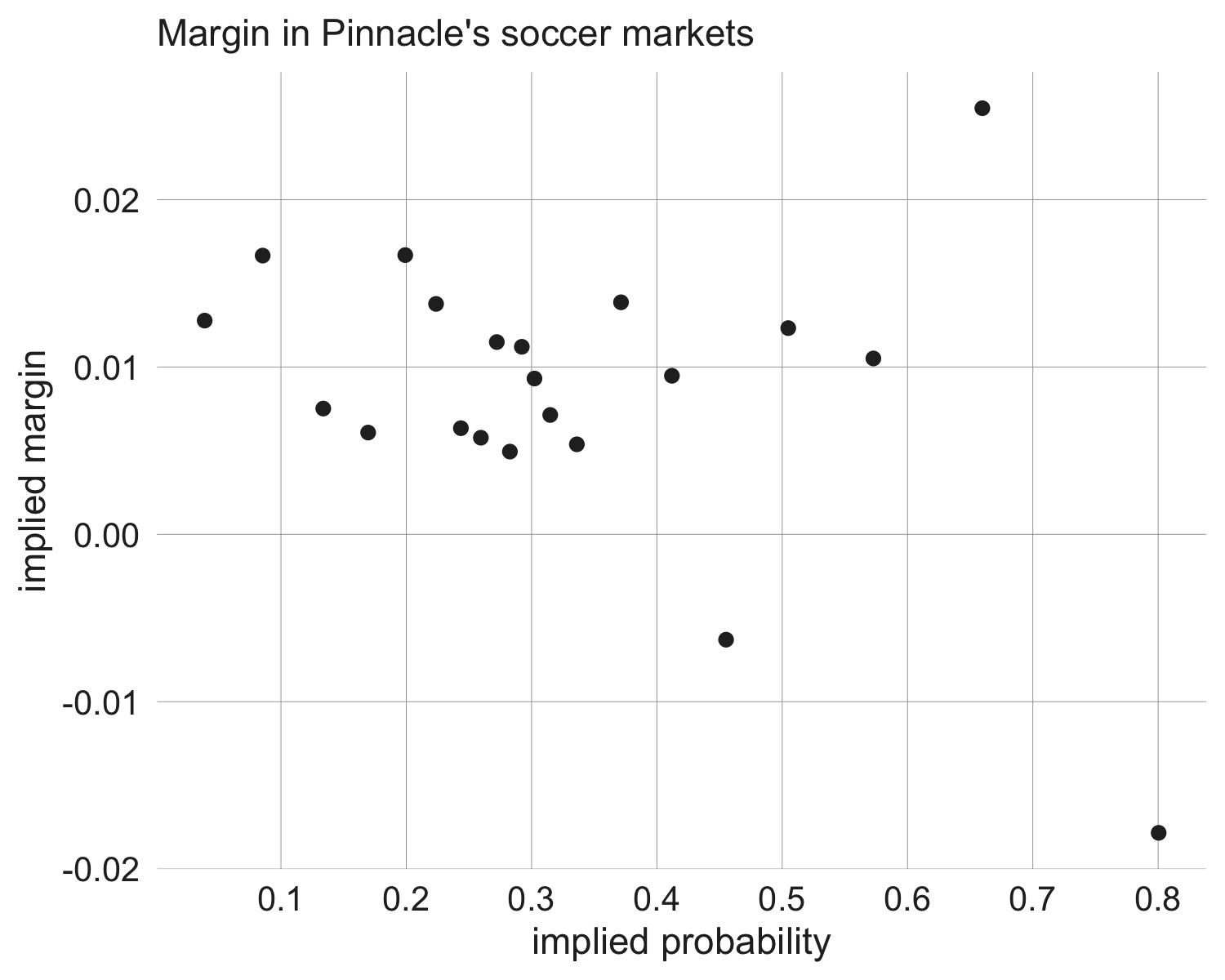
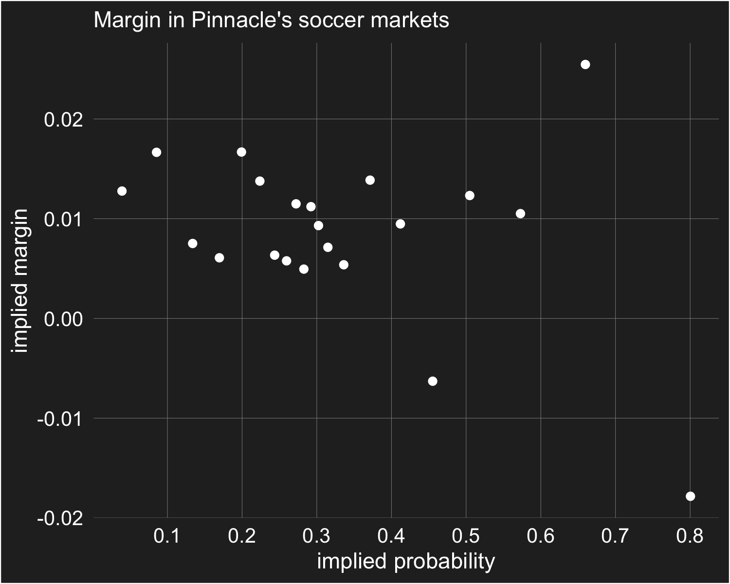
This first plot shows the average implied margin — equal to the
implied probability minus our estimate of the fair probability — as a
function of implied probability. To make things transparent, I've simply binned
the data (~4000 data points per bin) and calculated implied margin as the
average implied probability in that bin minus the average result in that bin.
For example, the 4000 longest
odds in the data, captured by the left-most data point in the plot below,
had an average implied probability of 0.0391, and 0.0263 of these
events in fact occurred; this implies an average margin of 0.0128.
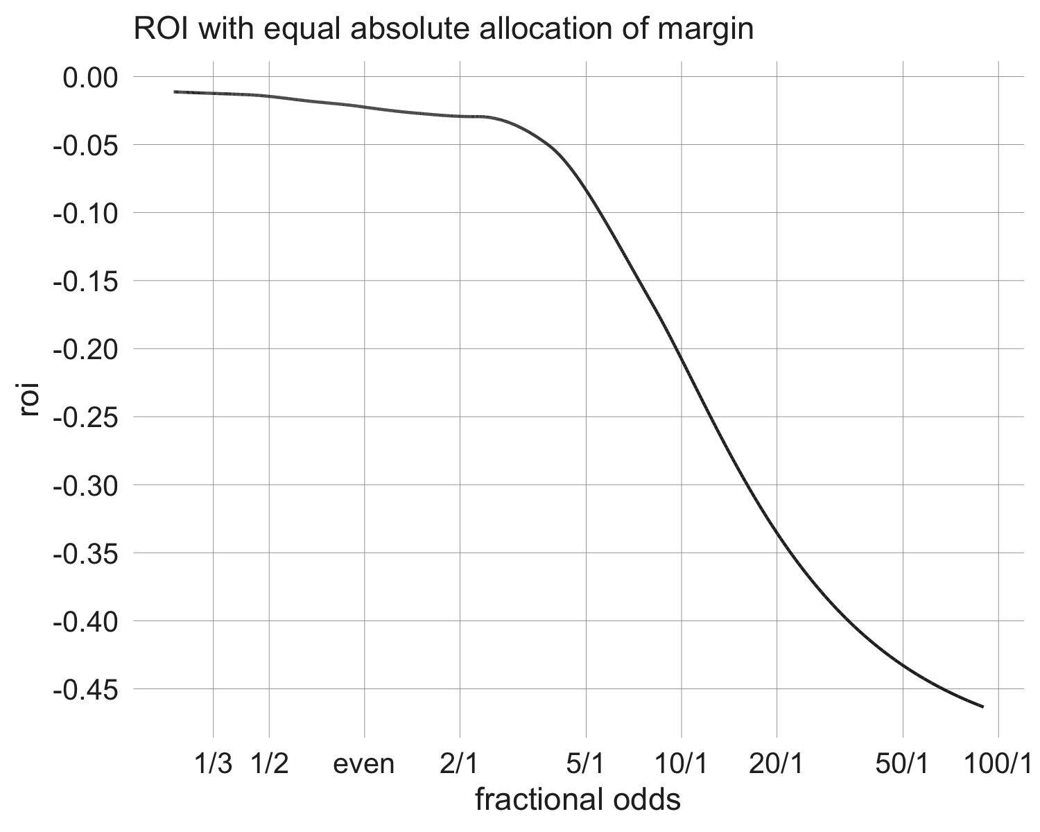
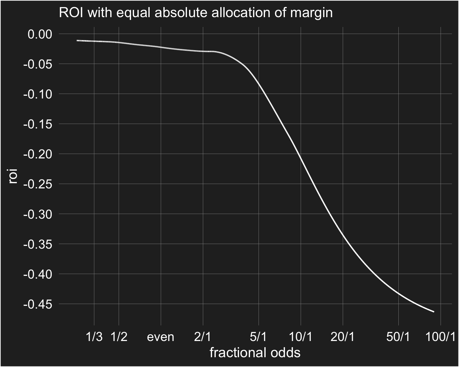
Next, we'll look at some of the data from one of the better-known papers on the FL bias: Wolfers and Snowberg 2010 (W&S). They motivate their paper with a plot of average returns as a function of the odds level, using data from over 5 million horse races in the US (p.1 of the linked pdf). As odds lengthen, the average rate of return declines drastically. The authors state that this illustrates that market prices are providing biased estimates of the probability of a horse winning. To make a statement like this requires some assumption about how the margin in the market should be removed. If you assume proportional margin allocation, as a risk-neutral representative bettor model predicts, then the claim follows. However, as is hopefully clear at this point, there is no reason to expect a margin to be allocated proportionally, and therefore no reason to conclude that the market provides biased probability estimates simply because returns decline as odds lengthen.
The plot below displays average returns as a function of odds (using the same log scale as W&S for the purpose of comparability) from simulated data with margin allocated equally. More specifically, I generate 100,000 "true" probabilities between 0.1% and 90% and add 1% to every price. I then simulate the result of each bet using the true probabilities and fit a smooth curve to rate of return as a function of price.
| odds | implied probability |
rate of return |
implied true probability |
implied margin |
|---|---|---|---|---|
| 1/3 | 0.750 | -0.09 | 0.683 | 0.067 |
| 1/2 | 0.667 | -0.10 | 0.600 | 0.067 |
| 1 | 0.500 | -0.15 | 0.425 | 0.075 |
| 2 | 0.333 | -0.17 | 0.276 | 0.057 |
| 5 | 0.167 | -0.19 | 0.135 | 0.032 |
| 10 | 0.091 | -0.20 | 0.073 | 0.018 |
| 20 | 0.048 | -0.23 | 0.037 | 0.011 |
| 50 | 0.020 | -0.40 | 0.012 | 0.008 |
| 100 | 0.010 | -0.58 | 0.004 | 0.006 |
| 200 | 0.005 | -0.64 | 0.002 | 0.003 |
In Pinnacle's soccer markets we observed a relatively constant margin allocation across the entire range of prices, while in W&S there is a sharp decline in margin at extreme probabilities. Therefore, in this respect, these margins are more consistent with the model presented in Section 3 than Pinnacle's. Even though we didn't observe it with Pinnacle's prices, it must be the case that the margin eventually declines as the true odds move close enough to 0 and 1. An important difference between these two markets to consider is that Pinnacle's soccer markets have very little margin (2-3% total on a 3-outcome market); contrast that with the horse racing markets in W&S, which have 6-7% margin on some individual prices. As probabilities move towards 0 and 1, Pinnacle's 0.8-1% margins on individual prices can be sustained a lot longer than these 6-7% margins.
My takeaways (and hopefully yours)
The empirical evidence for declining rates of return
at longer odds in gambling markets is
strikingly robust; indeed, it's so strong
that it should give you pause. If this pattern was the product of irrational
behaviour or non-standard preferences, it seems unlikely that it would be
as ubiquitous as it is.
From a theoretical standpoint, the finding of lower average returns at longer odds
is not interesting;
the simplest heterogeneous agent models that have been
used to model prediction markets can account for it.
The only class of model that seems capable of predicting equal rates of returns
across the range of possible prices
is that of the representative bettor. But, as I've argued in the preceding
sections, representative bettor models
are not suitable for modelling markets with non-zero margin.
A related empirical pattern is one typically associated with prediction markets: the midpoint of the bid-ask spread sometimes overestimates objective probabilities for low-probability events and underestimates it for high-probability events. In the framing of a traditional betting market, a bias in the midpoint of the bid-ask is equivalent to more margin being allocated to longshots than favourites in an absolute sense. This bias is nontrivial from a theoretical standpoint, and many interesting models have been proposed to explain it. However, the empirical evidence for the existence of this bias is not that strong. Some markets show it, but many don't. Both markets I analyzed in Section 4 don't display this pattern. However there are several examples of betting markets that exhibit positive returns at the shortest odds (which is obvious evidence of an FL bias in the bid-ask spread, or more margin being allocated to longshots). I think most high-volume betting markets will have margin allocated equally, as Pinnacle's soccer markets were shown to in the previous section. For more extreme prices, it's likely inevitable that the margin declines, however we should still expect equal margins at p and 1-p.
The most important takeaway from this blog post is a simple one: the two definitions of the favourite-longshot bias just described have been conflated by researchers. Most of the motivating empirical evidence for papers on the FL bias comes in the form of declining returns at longer odds, while most of the proposed theory is attempting to explain why a bias in the bid-ask spread might arise. The one setting where these two definitions of the FL bias are equivalent is when there is no margin in the market, and this is often the only case considered by researchers when developing a theoretical framework to rationalize the bias. This is one potential reason why this insight has slipped through the cracks. A second reason might be that research on bookmaker markets and prediction markets has been siloed to a large degree. As Section 2 showed, a binary prediction market can always be reframed as a traditional bookmaker market with only "win" contracts. This reframing makes it clear that the absence of a bias in the bid-ask spread implies that returns will decline as odds lengthen. The key implication of this conflation of definitions is that the evidence for the bias-in-the-midpoint version of the FL bias is not anywhere near as strong as we've presumed it is, because most of the empirical evidence is for the lower-returns-at-long-odds version of the bias. It seems everyone has taken evidence for the latter to be evidence for the former, when in fact that is not the case.
There is no question that declining returns at longer odds feels like a bias that needs explaining. Taking a broader view, the key characteristic of betting markets is that they are, in the aggregate, negative expected value for prospective bettors. As a result, the usual intuitions about risk-neutral arbitrage, i.e. if asset A returns more than asset B arbitrageurs will buy up A, which representative bettor models rely on, don't apply. For example, if a bettor came along who, having read the literature on the favourite-longshot bias, understood that better returns could be had by betting only on heavy favourites, would she employ that strategy? The answer is no, because the bettor, if risk-averse and rational, would be better off by simply not participating. On the other hand, suppose there was a betting market that had negative total margin; that is, on average bettors make money by participating. Then the logic of a risk-neutral representative bettor placing bets until returns are equalized across all offered bets actually makes sense, and unequal returns would be a puzzle (as would the mere existence of this market).
To conclude, consider the question to the answer in the title: does the fact that expected returns are lower at longer odds represent a market inefficiency? Market efficiency is an illusive concept. As stated in the seminal 1970 paper by Eugene Fama [5], an efficient market is one where prices "fully reflect" the available information. Differing degrees of efficiency are then defined on the basis of what is considered "available information". As Fama explains, to go from a claim about market efficiency to a claim about expected returns requires specifying the process of price formation in the market. When using a representative bettor framework, which is a particular model of price formation, prices must be set such that the bettor is indifferent to all offered bets, making lower returns at longer odds a sign of some inefficiency. Conversely, using a simple heterogeneous bettor model, which outlines a different process for price formation, declining returns at long odds says nothing about the efficiency of market prices. In the version of the model outlined in this post, the bookmaker knew the true event probability, while the bettors' beliefs were only correct on average. Whether this constitutes "full information" is up for debate; if both bookmakers and bettors knew the objective probabilities, a market with transaction costs could not exist. Therefore it seems this might be as close to full information as a real-world betting market could get. If you concede this, and agree that the heterogeneous bettor model is the most straightforward representation of a betting market, then it follows that the favourite-longshot bias — as it's traditionally defined — is not a market inefficiency or a bias.